
When analyzing resistor-inductor circuits, remember that current through an inductor cannot change instantaneously as this would require an infinite voltage source. When a circuit is first energized, the current through the inductor will still be zero, which is characteristic of opens. Once at steady-state, the current has leveled out and therefore the voltage across the inductor will approach zero, which is characteristic of shorts. Thus, we can state the general behavior of inductors at the beginning and ending of the charge cycle: \[\text
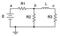
Assuming the initial current through the inductor is zero in the circuit of Figure 9.3.2 , determine the voltage across the 2 k\( \Omega \) resistor when power is applied and after the circuit has reached steady-state. Draw each of the equivalent circuits. 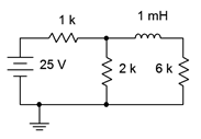 Figure 9.3.2 : Circuit for Example 9.3.1 . First, we'll redraw the circuit for the initial-state equivalent. To do so, open the inductor. The new equivalent is shown in Figure 9.3.3 . By opening the inductor, the 6 k\( \Omega \) resistor has been removed from the circuit and sees no voltage. What we are left with is a voltage divider between the source and the 1 k\( \Omega \) and 2 k\( \Omega \) resistors.
 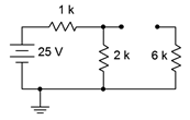 Figure 9.3.3 : Initial-state equivalent of the circuit of Figure 9.3.2 . Using the voltage divider rule, \[V_ = E \frac \nonumber \] \[V_ = 25 V \frac < 2k \Omega +1 k \Omega>\nonumber \] \[V_ \approx 16.67V \nonumber \] For steady-state, we redraw using a short in place of the inductor, as shown in Figure 9.3.4 . Here we have another voltage divider, this time between the 1 k\( \Omega \) resistor and the parallel combination of 2 k\( \Omega \) and 6 k\( \Omega \), or 1.5 k\( \Omega \).
 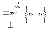 Figure 9.3.4 : Steady-state equivalent of the circuit of Figure 9.3.2 . \[V_ = E \frac \nonumber \] \[V_ = 25 V \frac < 1.5k \Omega +1k \Omega>\nonumber \] \[V_ = 15V \nonumber \]
To verify the results of Example 9.3.1 , the circuit is entered into a simulator as shown in Figure 9.3.5 . A DC operating point analysis is run and the results are shown in Figure 9.3.6 . 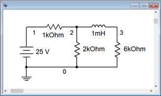 Figure 9.3.5 : Circuit of Figure 9.3.2 in a simulator. The steady-state potential at node 2 corresponds to the voltage across the 2 k\( \Omega \) resistor and agrees with the theoretical calculation of 15 volts. Note that node 3 is also 15 volts, indicating that the steady-state voltage across the inductor is zero, meaning it is behaving as a short, exactly as expected.
 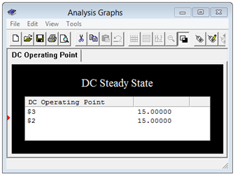 Figure 9.3.6 : Simulation results for the circuit of Figure 9.3.2 .
This page titled 9.3: Initial and Steady-State Analysis of RL Circuits is shared under a CC BY-NC-SA 4.0 license and was authored, remixed, and/or curated by James M. Fiore via source content that was edited to the style and standards of the LibreTexts platform.